
Reactor Kinetics Equations applied to the start-up
phase of a Ringhals PWR
by Frigyes Reisch
Classical reactor kinetic equations with six
groups of delayed neutrons (point kinetics) are not solved analytically.
In the following programme the fuel and the moderator thermal
dynamic equations are coupled to the reactor kinetic equations.
The equation system is solved numerically with MATLAB and applied
to a Ringhals PWR‘s start-up phase at zero power operation,
when the fuel and moderator temperature increase is very modest.
The results are presented graphically.
The programme can, of course, also be used for
low power operation with some changed input data - and for various
other reactors too.
This short programme with changed parameters
is also suitable for nuclear engineering students to use when
training at research reactors.
The calculations and the measured data are in agreement.
Fredrik Winge, a reactor physics specialist in
Ringhals, supplied the chart with the measured data and was an
invaluable partner.
The simplified neutron kinetics equations

|
or |
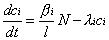 |
Here
t |
time (sec) |
N |
neutron flux (proportional to the reactor power) |

|
change of the effective neutron multiplication factor
(keff) |
ß |
sum of the delayed neutron fractions (here 0.006502) |
ßi |
the i:th delayed neutron fraction |
l |
neutron mean lifetime (here 0.001 sec) |

|
i:th decay constant (sec-1) |
| ci |
concentration of the i:th fraction of the delayed neutrons’
precursors,
At steady state, when time is zero t=0 all time derivatives
are equal to zero, all d/dt=0 and the initial value of the
relative power equals unity N(0)=1, and also no reactivity
perturbation is present =0
|
Delayed neutron data for thermal fission in
U235 is used as follows:
| Group |
1 |
2 |
3 |
4 |
5 |
6 |
Fraction ßi |
0.000215 |
0.001424 |
0.001274 |
0.002568 |
0.000748 |
0.000273 |
Decay constant |
0.0124 |
0.0305 |
0.111 |
0.301 |
1.14 |
3.01 |
The initial values of the delayed neutrons’
precursors are as follows:
| i |
1 |
2 |
3 |
4 |
5 |
6 |
| ci(0) |
17.3387 |
46.6885 |
11.4775 |
8.5316 |
0.6561 |
0.0907 |
Using the MATLAB notations
x(1)=N x(2)=c1…………
x(7)=c6
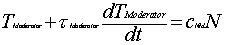
Fuel
The fuel temperature change (TFuel) follows
after the power
with a time delay ( )
)
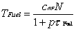
Where:
TFuel |
Fuel temperature change |
| N |
Relative neutron flux proportional to the relative power
cFN fuel temperature proportionality constant
to relative power |
p |
Laplace operator d/dt, 1/sec |
|
thermal time constant of the fuel, here 5 sec |
t |
time, sec |
The differential equation form is
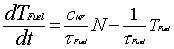
At a steady state (equilibrium) d/dt=0 N(0)=1
Suppose that at zero power the fuel temperature changes by 0.001
0C when N=1 and, therefore, cFN=0.001
Suppose |
|
=5 sec |
 |
=0.2 |
 |
=0.00020C/sec |
With the MATLAB notation x(8) = TFuel
and the neutron kinetics equations can be expanded to include
the fuel dynamics
0.0002*x(1)-0.2*x(8)
The Doppler reactivity of the fuel is
Here

|
The reactivity contribution of the fuel temperature
change, at the initial phase (t=0), at steady state (equilibrium)
is zero: 
|

|
Fuel temperature coefficient (Doppler coefficient) here
is -3.1pcm/0C |
The reactivity of the Fuel’s Doppler effect
is
|
= |
|
( ) ) |
= -3.1 10-5 .(TFuel
- 0.001) |
with MATLAB notation
DeltaKfuel = – 3.1.10-5*x(8) + 0.0031.10-5
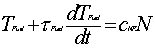
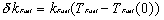
Moderator
The differential equation for the moderator is
similar to that of the fuel, when the moderator thermal time constant
is much bigger then the fuel thermal time constant:

|
>> |
 |
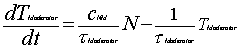
| TModerator |
Moderator temperature change |
|
Moderator thermal time constant, here 100
sec |
| cNM |
Moderator temperature proportionality
constant to the relative power, supposing that at zero power
operation the moderator temperature change is only 0.0005
0C when the relative power N=1. Then cNM=0.0005 |
| Suppose |
|
=
100sec |
 |
=0.01/sec |
 |
=
0.0005.0.01 0C/sec =0.000005 |
With the MATLAB notation x(9) = TModeratorl
The neutron kinetics equations can be expanded to
include the moderator dynamics too:
0.000005*x(1)-0.01*x(9)
Moderator reactivity contribution from temperature
change

Here

|
the reactivity contribution of the moderator
temperature change at the initial phase (t=0), at steady
state (equilibrium) is zero 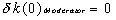 |

|
Moderator temperature coefficient here is - 0.6pcm/0C |
The reactivity contribution from the changing moderator
temperature is as follows:
with MATLAB notation
DeltaKmoderator=-0.6.10-5*x(9)+0.0003.10-5
Control Rods
| 
|
the reactivity contribution
of the control rods’ movement - here with the maximum
value of 50 pcm (~8 cent, 1$˜650 pcm)
The movements of the rods and the corresponding reactivity
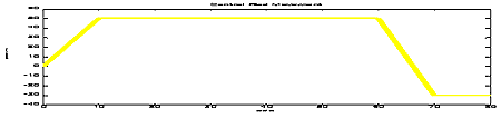
changes are given in the first and third chart
|
The reactivity balance with the control rods,
the fuel’s Doppler effect and the moderator’s temperature
effect is

The reactivity balance with MATLAB notation
DeltaK = DeltaKcr + DeltaKfuel + DeltaKmoderator
Comparison with Measured Data
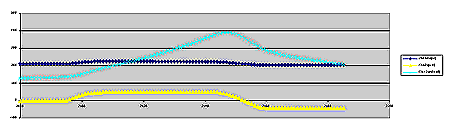
The first chart indicates the
measured data, the neutron flux is shown by the light blue curve.
The control rod reactivity is represented by the yellow curve.
The dark blue dots indicate the control rod steps.
In the second chart, the calculated relative
neutron flux is displayed and the curve is pretty much in agreement
with the measured data.
In the third chart, the schematic of the control
rod reactivity used in the calculations is indicated.
In the fourth chart, the characteristics
of the fuel and moderator temperature increase are shown. The
values are very small as on this occasion the calculations are
performed for zero power operation, when practically no power
is generated in the fuel and transferred to the moderator. However,
the curves clearly demonstrate that the fuel’s thermal time
constant is much smaller than that of the moderator’s.
1st chart, measured data
2nd chart, calculated relative neutron flux

3rd chart, schematic of the control rod reactivity
4th chart, characteristics of the fuel and moderator
temperature increase

The code
The code contains two parts:
Part one
%Save as xprim9FM.m
function xprim = xprim9FM(t,x,i)
DeltaKcr=i*10^-5;
DeltaKfuel=-3.1*10^-5*x(8)+0.0031*10^-5;
if t>=0 & t<10
DeltaKcr=((i*10^-5)/10)*t;
end
if t>60 & t<70
DeltaKcr=(10^-5)*(i-8*(t-60));
end
if t>70
DeltaKcr=-30*(10^-5);
end
DeltaKmoderator=-0.6*10^-5*x(9)+0.0003*10^-5;
DeltaK=DeltaKcr+DeltaKfuel+DeltaKmoderator;
xprim=[(DeltaK/0.001-6.502)*x(1)+0.0124*x(2)+0.0305*x(3)+0.111*x(4)+0.301*x(5)+1.14*x(6)+3.01*x(7);
0.21500*x(1)-0.0124*x(2);
1.424000*x(1)-0.0305*x(3);
1.274000*x(1)-0.1110*x(4);
2.568000*x(1)-0.3010*x(5);
0.748000*x(1)-1.1400*x(6);
0.273000*x(1)-3.0100*x(7);
0.000200*x(1)-0.2000*x(8);
0.000005*x(1)-0.0100*x(9)];
Part two
%Save as ReaktorKinFM.m
figure
hold on
for i=50 %i is the max Control Rod reactivity i pcm
[t,x]=ode45(@xprim9FM,[0 80],[1; 17.3387; 46.6885; 11.4775; 8.5316;
0.6561; 0.0907;0.001; 0.0005],[] ,i);
plot(t,x(:,1:1))
end
hold off
|